Lab- Find the focal length of a convex lens
Pre-lab Questions
• What is the difference between a real and a virtual focus?
• What is a lens?
• What is the principle axis of a mirror, of a lens?
• What is the difference between a real and a virtual image?
• What is a virtual object?
• What does the relative size of object and image depend on?
• What is the difference in the convention for mirrors and the convention for lenses?
Procedure
Measure the focus of a real lens. Using a source far away (several meters) find the point where the image of this distant source is brought to a focus on a screen. With the room lights dimmed use the light coming through the lab door or window as an object. How does this compare with the value printed on the lens housing?
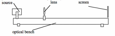
Place the optical source at one end of the optical bench and place the white screen on the opposite end of the optical bench. Place a convergent lens between the source and the screen but nearer to the source and find the spot where a focused image of the source is projected onto the screen. Observe that the image is larger than the source because the image distance is larger than the source distance to the lens. Note the position of the lens. Measure the object distance do and the image distance di and use them in the formula
1/do + 1/di = 1/f
to find the focal length of the lens. Is it comparable to the value observed above? Is it similar to the previously observed values?
Lab Setup
• What is the difference between a real and a virtual focus?
• What is a lens?
• What is the principle axis of a mirror, of a lens?
• What is the difference between a real and a virtual image?
• What is a virtual object?
• What does the relative size of object and image depend on?
• What is the difference in the convention for mirrors and the convention for lenses?
Procedure
Measure the focus of a real lens. Using a source far away (several meters) find the point where the image of this distant source is brought to a focus on a screen. With the room lights dimmed use the light coming through the lab door or window as an object. How does this compare with the value printed on the lens housing?
Place the optical source at one end of the optical bench and place the white screen on the opposite end of the optical bench. Place a convergent lens between the source and the screen but nearer to the source and find the spot where a focused image of the source is projected onto the screen. Observe that the image is larger than the source because the image distance is larger than the source distance to the lens. Note the position of the lens. Measure the object distance do and the image distance di and use them in the formula
1/do + 1/di = 1/f
to find the focal length of the lens. Is it comparable to the value observed above? Is it similar to the previously observed values?
Lab Setup
Lab- Thin Lens
3.2 Measuring the Focal Length – II
Place an object on one side of the lens and a mirror on the other side, as indicated in the figure below.
Place an object on one side of the lens and a mirror on the other side, as indicated in the figure below.
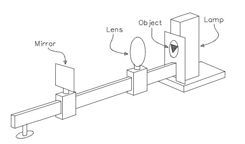
When the object is in the focal plane of the lens (i.e., when S = f) all
the rays from a point on the object, which pass through the lens, will
emerge in a parallel bundle (much like the figure shown in section 2.1).
The rays remain parallel after reflection from the mirror. Any
reflected parallel bundle will then pass back through the lens and
converge at a point in the original focal plane. The location of the
focal plane can thus be determined by varying the object-to-lens
distance until a sharp image is formed on the object screen it- self,
where the object-to-lens distance just equals the focal length. By using
the backlit small triangular screened opening as an object, you can
observe the image superimposed on the object and move the lens until the
image is sharp.
3.3 Lens Equation
Use the same setup as in section 3.2 but instead of the mirror, use a screen. Locate the lens more than a focal length away from the object and adjust the position of the screen until you get a sharp image on the screen. By measuring S and S', you can verify the lens equation.
With several measurements of S and S', make a 1/S vs. 1/S' graph and estimate a best-fit line. This permits a measure of the focal length to compare with your previous result.
Lab- Telescopes
In this lab, you will study the optical properties of telescopes, eyepieces, and field lenses on the optical bench. In the first labs, you started with a clear optical table and set up all of the optics yourself; in this week’s lab, there will be some equipment set up on each bench. You’ll spend the first day at one setup (Part I or II), then switch places for the second day.
Part I : Telescope imaging
The preliminary setup here features a 50 mm diameter, 260 mm focal length achromatic doublet collimator sending light from a test target into a 6-inch aperture Maksutov-Cassegrain telescope attached (somewhat precariously) to the optical table. The test target is illuminated by the QTH lamp from lab #1, but with a white opal glass diffuser between the lamp and the target for more even illumination. In addition to this write-up, there is also a handout of describing the pattern element line spacings for the USAF resolution test target. The telescope is equipped with a micrometer eyepiece that contains a moving crosshair to measure the size of image features in the telescope focal plane. Turn on the QTH lamp and record the measurements below in your lab notebook.
Measurements. Once you have learned how to read the test target patterns, use the micrometer eyepiece to measure the sizes of an element (one “line pair”) in each group that is visible. You know from the “Line Pairs Per Millimeter” chart the actual sizes of each feature measured in the focal plane of the 260mm lens, so from your measurements you can determine the effective focal length (EFL) for the 6-inch telescope. Note that underneath the telescope at the eyepiece end is a small knob to be used for focus; make all of your micrometer measurements at a single telescope focus setting.
Remove the eyepiece and eyepiece holder—the first just pulls out, while the holder is threaded into the telescope tube. Likewise remove the threaded cap in the center of the eyepiece end of the telescope. With these parts removed, describe in your notebook the function of the two knobs at the back end of the telescope. Is the lens carried into position below the eyepiece a positive or negative lens? What will be the effect of this lens on the effective focal length of the telescope? Return the knobs to their original positions, and replace the parts you have removed. Move the knob that controls the motion of the lens inside the tube, and observe the result by looking into the eyepiece. Move the knob that controls the motion of the lens, and observe the result by looking into the eyepiece (turning the focus knob for sharpest focus). Does the result confirm your expectation? Using the micrometer eyepiece again, re-measure at least one line pair spacing on the target to re-determine the effective focal length of the telescope plus lens.
1
Replace the micrometer eyepiece with the 40 mm, 15 mm, and 10.8 mm effective focal length eyepieces and record the target appearance for each. What is the outermost group you can see, what is the smallest element you can resolve with your eye, etc. Note that you may need to refocus the telescope for different eyepieces.
Turn off the QTH lamp and put a white screen in front of the entrance to the telescope; room light should illuminate the side of the screen facing the telescope. With a second opal glass or ground glass diffuser, locate the exit pupil formed by each of the 40 mm, 15 mm, and 10.8 mm eyepieces and measure the diameter of this exit pupil as accurately as you can.
Analysis. For each of your USAF test target measurements, calculate the angle subtended by a line pair in the focal plane of the 260 mm lens and use this angle together with your micrometer measurement to determine the EFL of the telescope. Use your error estimates to compute a weighted mean average for the telescope EFL. When the full 6-inch aperture of the telescope is used, what is the effective f/ratio of the telescope? What happens to the EFL and f/ratio when the small lens is inserted into the beam beneath the eyepiece holder?
Calculate the angular magnifications achieved with the 40 mm, 15 mm, and 10.8 mm eyepieces. Dividing the 6-inch aperture by the magnification, predict the exit pupil diameter and compare the values you measured. What angular magnifications and pupil diameters would you have found if the additional lens were used?
Part II : Reimaging Systems and Pupils
This lab was originally designed to be performed with the use of two HeNe lasers, spatial filters, and 50 mm diameter laser collimators on the optical table. However, if you tried to make a large diameter colimated laser beam in Lab 1, you can recall that the equipment is very fragile and the slightest bump can ruin the alignment. Therefore, for the sake of efficiency, this lab can be done using colimated light of QTH lamps, as in Lab 1. You can try to set up a collimated broad laser beam, if you have unusual mechanical aptitude, plenty of time, and a lot of patience.
You will notice that one beam is aligned with the long optical rail and will this be “on-axis” for any optics on the right side of the rail. The other collimated beam is at the same height above the table but is aligned at an “off-axis” angle with respect to the long rail. You will use these two beams to simulate on-axis and off-axis ray bundles to study focal planes, field lenses, and pupils.
For tracking the beams more esily, we can also place different filters in front of the lamps (for example, a “green” filter for the “on-axis” beam and a“red” filter for the “off-axis” one).
Measurements. Begin by observing the collimated beams as they intersect and move apart. Estimate the rail scale reading that corresponds to the point of intersection. Install the Nikon lens and carrier so that the two beams intersect in the middle of the lens body. In your lab notebook, record the focal length of the lens (written around the front of the lens), and set the f/stop ring of the lens to a focal ratio of f/5.6. You should feel the lens click into this stop position; you may need to rotate part of the lens if it is mounted by the f/stop ring. Set the lens focus to ∞.
Locate the focal plane of the lens and measure the separation between the “on- axis” and “off-axis” image by using the ruler as a screen. Measure the reading on the rail scale corresponding to the focal plane.
Turn your attention next to the patterns on the wall. Use the ruler to extrapolate the optical rail scale reading to the wall., and record the reading that corresponds to the wall position. Recall from lecture the discussion of the “chief ray” that passes through the center of the aperture stop, and therefore is located at the center of the ray bundles. Measure the distance on the wall separating the chief rays of the on-axis and off-axis beams. Also measure the diameters of the two patches on the wall.
Calculate ∆x between your optical rail scale readings for the focal plane and the wall, and the ∆y between the separations of the foci and the patches on the wall. Make a scale layout in your lab notebook of the xy-plane and draw rays between the foci and the wall patches, then extrapolate backwards the off-axis chief ray and the optical axis until they intersect. Describe what occurs at (and what name is given to) this intersection point. Calculate the x-coordinate of this location where ∆y = 0.
Install the EFL = 80 mm mounted f/2.8 air-spaced triplet lens behind the Nikon lens, and focus to reimage the foci onto the wall. What happens to the off-axis beam? Record the EFL = 80 mm lens carrier scale reading where the on-axis beam is focused on the wall, and also record your observations pertaining to the off-axis beam.
Next locate a 33 mm diameter, 57 mm focal length plano-convex “field lens” at the Nikon lens focus. Move the 80 mm focal length triplet out of the way, and observe the behavior of the on- and off-axis ray bundles following the field lens. Return the 80 mm focal length f/2.8 triplet to a position where images are focused on the wall, and record the lens carrier scale reading. Measure also the y-separation between the red and green images on the wall, and sketch these in your notebook. Finally, substitute the 36 mm diameter, 41 mm focal length double-convex “field lens” in place of the 33x57 lens in the Nikon lens focal plane and repeat the measurements in this paragraph.
Analysis. Determine the angular separation of the green and red beams as they enter the Nikon lens, and again as they leave (in this case, the angle between the optical axis as defined by the center of the green cone of light and the off-axis chief ray defined by the center of the red cone of light). Where inside the Nikon lens is the aperture stop as viewed from the focal plane, and what diameter is this aperture stop? Do your calculations based on the 57 mm and 41 mm field lenses agree for the location and diameter of the aperture stop inside the Nikon lens? What are the angles between the
optical axis and the off-axis chief ray following each of the field lenses?
Discussion
Summarize in your own words what you’ve learned in this lab about image scales, aperture stops, entrance and exit pupils, and how as an optical re-imaging instrument designer you can exert control over the location and direction of off-axis ray bundles. What are some of the penalties for ill-placed pupils in a re-imaging instrument? Provide examples to illustrate your points.
(If you find yourself lacking an example, consider the Palomar 200-inch diameter Hale Telescope, which has a Cassegrain f/ratio of f/16, and say you wanted to reimage the f/16 focal plane onto a CCD detector array that is 2048 by 4096 pixels on a side with 15 μm square pixels. In the reimaged focal plane you want 3 pixels per arcsecond on the sky. Think about pupil positions and sizes, and what effect a field lens would have.)
